Editor’s Note
Everyone I know uses Excel to some extent, but few (including me!) even scratch the surface of its capabilities. In this article, written by Ellen Su, Finance Expert at Toptal, the capabilities of Excel’s PowerPivor addin are demonstrated to provide a number of time saving analysis techniques. The original post can be read here.
Ellen is a fixed-income trader and portfolio manager who now freelances in financial modeling. She is excited to bring to Toptal clients a vast set of tools to employ on analytical projects. Her unique talent is a seamless combination of data sourcing, programming, financial analysis, storyboarding, and visualization.
Every financial analyst is a whiz with Excel. However, as storage becomes cheaper, our organizations are accumulating more data. And ever-more data makes it harder to work with Excel—we either reach the 1,048,576 row hard limit, or the document slows to a crawl trying to process everything.
Often, the decision is whether to lose some of the carefully curated details, or to work in a tediously slow workbook. Sometimes, we have to get creative in order to combine two large datasets. We resort to using convoluted formulas and waiting forever for the calculations to be resolved.
Fortunately, you no longer have to make these decisions. Excel’s Power Pivot functionality provides a way to extract, combine, and analyze large datasets. Despite the fact that it was released with Excel 2010, most financial analysts I meet still do not know how to use Power Pivot, and many do not know it even exists.
In this article, I will show you how to use Power Pivot to overcome common Excel issues, and take a look at additional key advantages of the software using some examples. This Power Pivot for Excel tutorial is meant to serve as a guide to what you can achieve with this tool, and at the end, I will explore some sample use cases where Power Pivot could prove invaluable.
What Is Power Pivot and Why Is It Useful?
Power Pivot is a feature of Microsoft Excel that was introduced as an add-in to Excel 2010 and 2013, and is now a native feature for Excel 2016. As Microsoft explains, Power Pivot for Excel “enables you to import millions of rows of data from multiple data sources into a single Excel workbook, create relationships between heterogeneous data, create calculated columns and measures using formulas, build PivotTables and PivotCharts, and then further analyze the data so that you can make timely business decisions without requiring IT assistance.”
The primary expression language that Microsoft uses in Power Pivot is DAX (Data Analysis Expressions), although others can be used in specific situations. Again, as Microsoft explains, “DAX is a collection of functions, operators, and constants that can be used in a formula, or expression, to calculate and return one or more values. Stated more simply, DAX helps you create new information from data already in your model.” Fortunately for those already familiar with Excel, DAX formulas will look familiar, since many of the formulas have a similar syntax (e.g., SUM, AVERAGE, TRUNC).
For clarity, the key benefits of using Power Pivot vs. basic Excel can be summarized as the following:
- It lets you import and manipulate hundreds of millions of rows of data where Excel has a hard constraint of just over a million rows.
- It allows you to import data from multiple sources into one single source workbook without having to create multiple source sheets that suffer from version control and transferability issues.
- It lets you manipulate the imported data, analyze it, and draw conclusions without slowing down your computer to a snail’s pace.
- It lets you visualize the data with PivotCharts and Power BI.
In the following sections, I’ll run through each of the above and show you how Power Pivot for Excel can be helpful.
1) Importing Large Datasets
As discussed previously, one of the major limitations of Excel pertains to working with extremely large datasets. Fortunately for us, Excel can now load well over the one-million row limit directly into Power Pivot.
To demonstrate this, I generated a sample dataset of two years’ worth of sales for a sporting goods retailer with nine different product categories and four regions. The resulting dataset is two million rows.
Using the Data tab on the ribbon, I created a New Query from the CSV file (Exhibit 1). This functionality used to be called PowerQuery, but as of Excel 2016, it is more tightly integrated into the Data tab of Excel.
Exhibit 1: Creating a New Query

From a blank workbook in Excel to loading all two million rows into Power Pivot, it took about one minute! Notice that I was able to perform some light data formatting by promoting the first row to become the column names. Over the past few years, the Power Query functionality has vastly improved from an Excel add-in to a tightly integrated part of the Data tab on the toolbar. Power Query can pivot, flatten, cleanse, and shape your data through its suite of options and its own language, M.
2) Importing Data from Multiple Sources
One of the other key benefits of Power Pivot for Excel is the ability to easily import data from multiple sources. Previously, many of us created multiple worksheets for our various data sources. Often, this process involved writing VBA code and copy/pasting from these disparate sources. Fortunately for us, though, Power Pivot allows you to import data from different data sources directly into Excel without having to run into the issues mentioned above.
Using the Query function in Exhibit 1, we can pull from any of the following sources:
- Microsoft Azure
- SQL Server
- Teradata
- Salesforce
- JSON files
- Excel workbooks
- …and many more
Further, multiple data sources can be combined either in the Query function or in the Power Pivot window to integrate data. For example, you can pull production-cost data from an Excel workbook and actual sales results from SQL server through the Query into Power Pivot. From there, you can combine the two datasets by matching production-batch numbers to produce per-unit gross margins.
3) Working with Large Datasets
Another key advantage of Power Pivot for Excel is the ability to manipulate and work with large datasets to draw relevant conclusions and analysis. I’ll run through a few common examples below to give you a sense of the power of the tool.
Measures
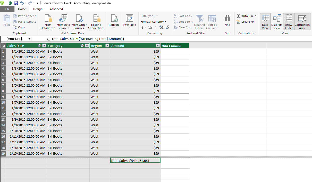
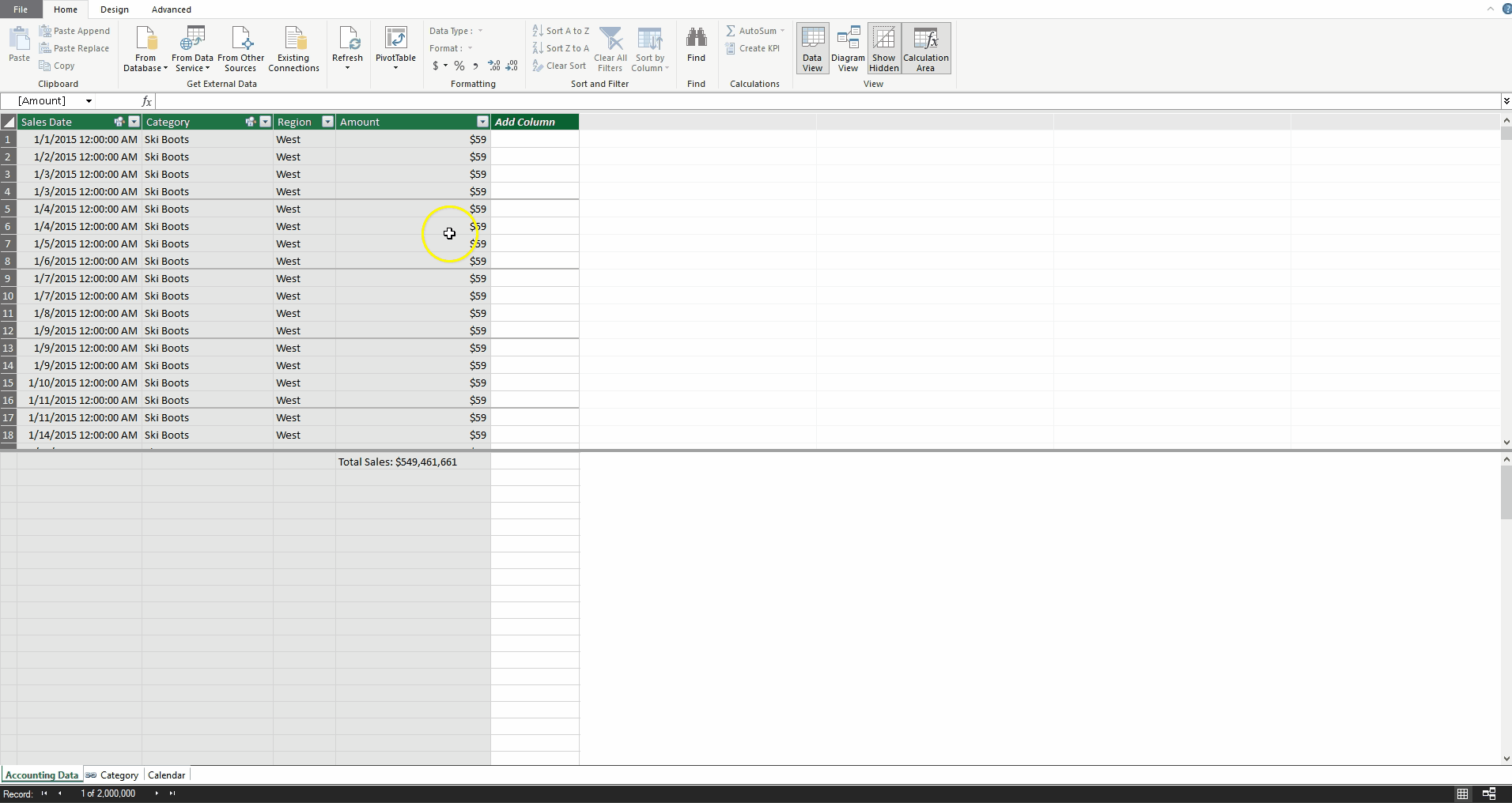
Excel junkies will no doubt agree that PivotTables are both one of the most useful, and at the same time, one of the most frustrating tasks we perform. Frustrating particularly when it comes to working with larger data sets. Fortunately, Power Pivot for Excel allows us to easily and quickly create PivotTables when working with larger sets of data.
In the image below (Exhibit 2), notice how the Power Pivot window is separated into two panes. The top pane has the data, and the bottom pane houses the measures. A measure is a calculation that is performed across the entire dataset. I have entered a measure by typing in the highlighted cell.
Total Sales:=SUM('Accounting Data'[Amount])
This creates a new measure that sums across the Amount column. Similarly, I can type another measure in the cell below
Average Sales:=AVERAGE('Accounting Data'[Amount])
Exhibit 2: Creating Measures
From there, watch how quickly it is to create a familiar PivotTable on a large dataset.
Exhibit 3: Creating a PivotTable

Dimension Tables
As financial analysts using Excel, we become adept at using convoluted formulas to bend the technology to our will. We master VLOOKUP, SUMIF, and even the dreaded INDEX(MATCH()). However, by using Power Pivot, we can throw much of that out the window.
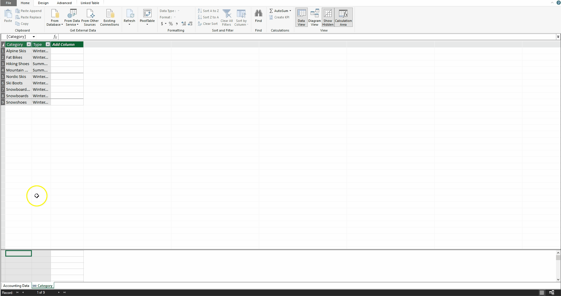
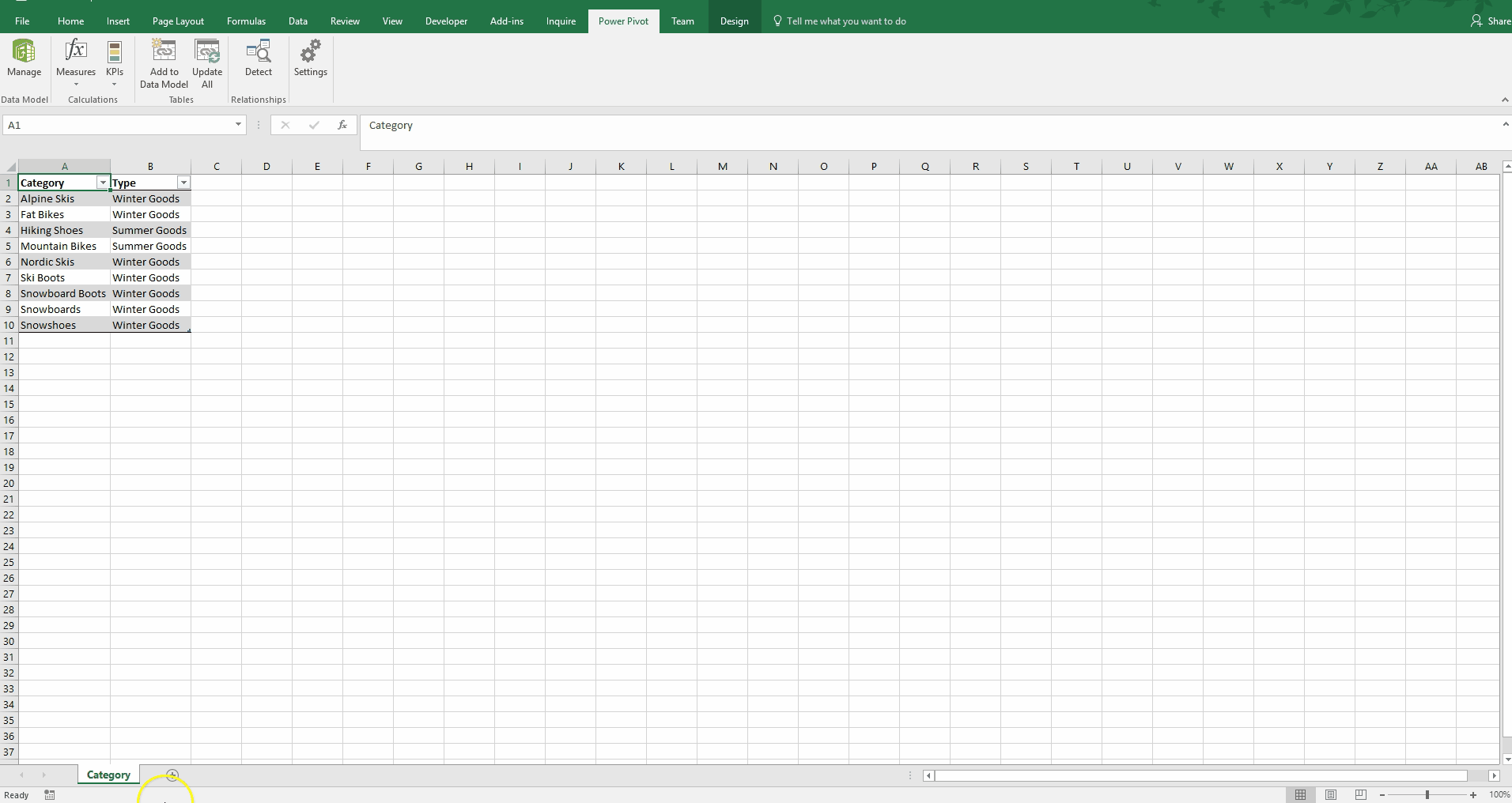
Exhibit 4: Adding a User-Created Table to a Power Pivot Model
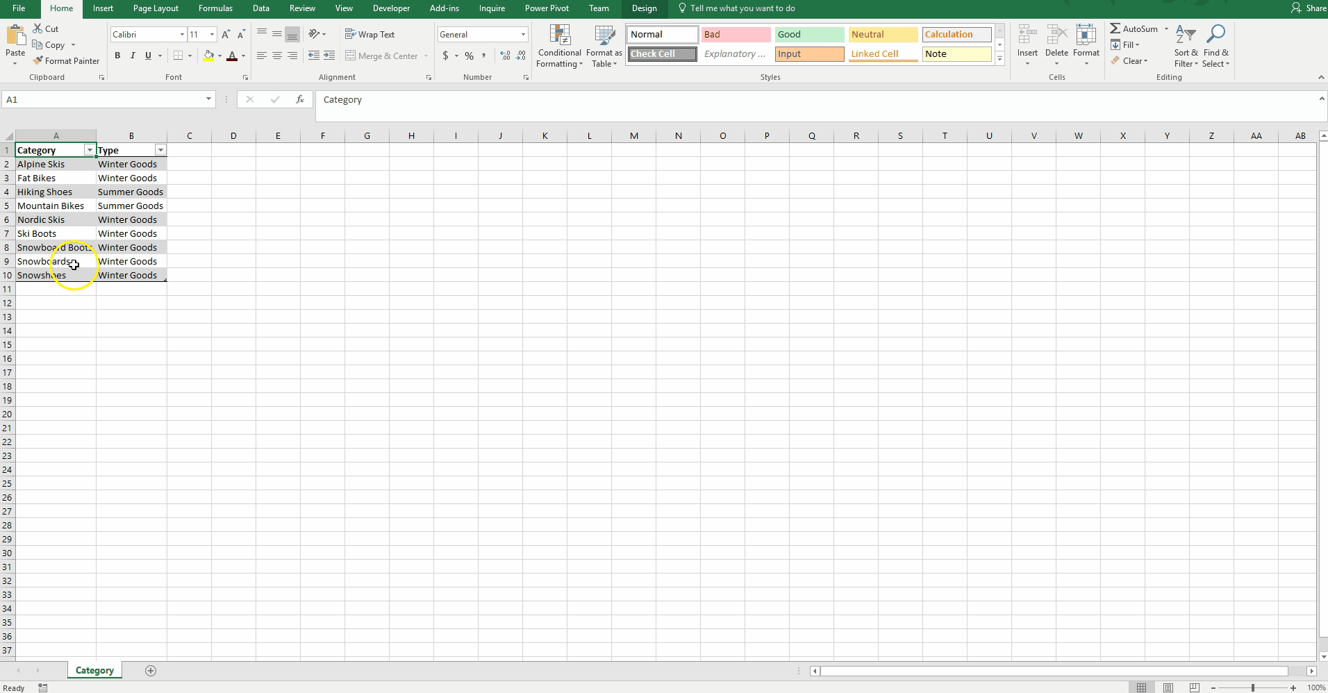
To demonstrate this functionality, I created a small reference table in which I assigned each Category to a Type. By choosing “Add to Data Model,” this table is loaded into Power Pivot (Exhibit 4 above).
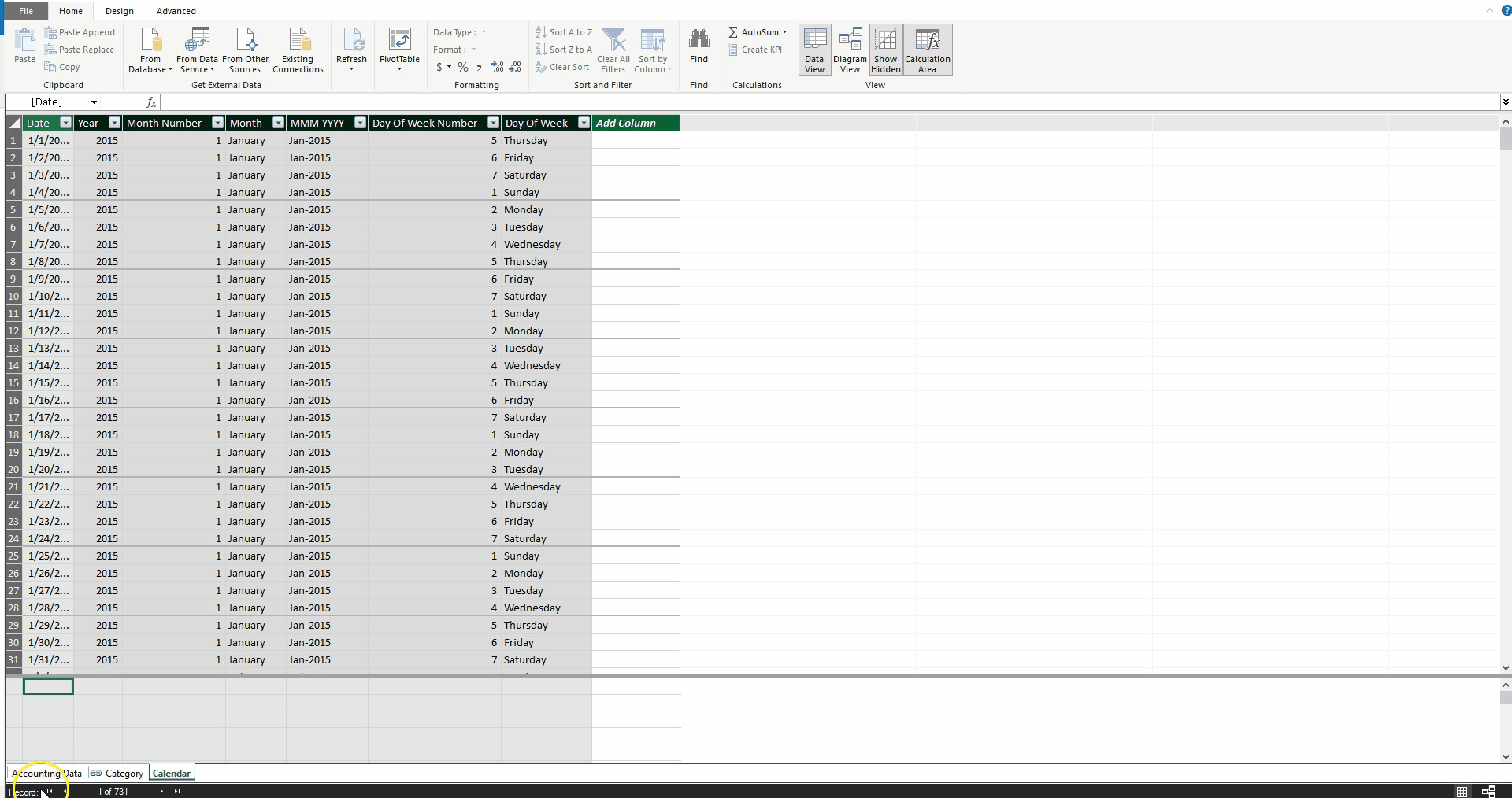
I also created a date table to use with our dataset (Exhibit 5). Power Pivot for Excel makes it easy to create a date table quickly in order to consolidate by months, quarters, and days of the week. The user can also create a more custom date table to analyze by weeks, fiscal years, or any organization-specific groupings.
Exhibit 5: Creating a Date Table
Calculated Columns
Besides measures, there is another type of calculation: calculated columns. Excel users will be comfortable writing these formulas, as they are very similar to writing formulas in data tables. I have created a new calculated column below (Exhibit 6) which sorts the Accounting Data table by Amount. Sales below $50 are labeled “Small,” and all others are labeled “Large.” Doesn’t the formula feel intuitive?
Exhibit 6: Creating a Calculated Column
Relationships
We can then create a relationship between the Accounting Data table’s Category field and the Category table’s Category field using the Diagram View. Additionally, we can define a relationship between the Accounting Data table’s Sales Date field and the Calendar table’s Date field.
Exhibit 7: Defining Relationships
Now, without any SUMIF or VLOOKUP functions needed, we can create a PivotTable that calculated Total Sales by year, and type, with a slicer for Transaction Size.
Exhibit 8: PivotTable Using Relationships
Or, we can create a chart of Average Sales for each day of the week using the new Calendar table.
Exhibit 9: PivotChart Using Relationships
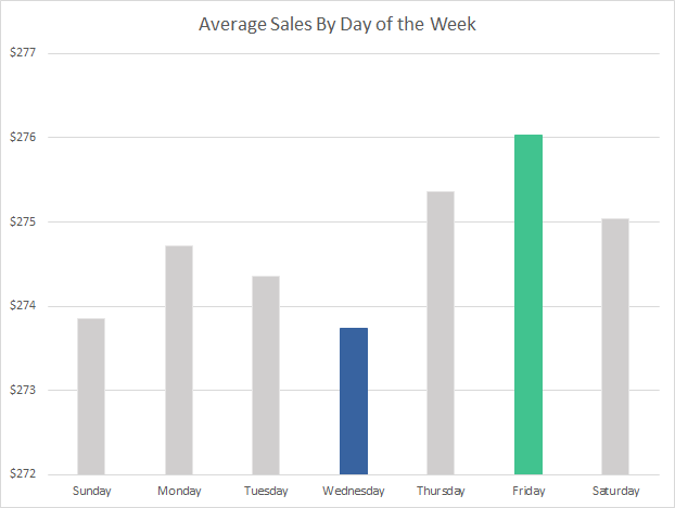
While this chart looks simple, it is impressive that it took less than ten seconds to create a consolidation over two million rows of data, without adding a new column to the sales data.
While being able to perform all these consolidated reporting scenarios, we can always still drill down into the individual line items. We retain our highly granular data.
Advanced Functions
So far, most of the analysis I have shown are relatively straightforward calculations. Now, I want to demonstrate the some of the more advanced capabilities of this platform.
Time Intelligence
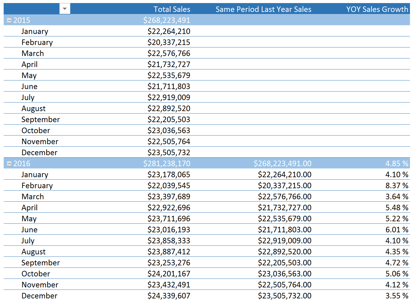
Often, when we examine financial results, we want to compare it to a comparable timeframe from the previous year. Power Pivot has some built-in time intelligence functions.
Same Period Last Year Sales:=CALCULATE([Total Sales],SAMEPERIODLASTYEAR('Calendar'[Date]))

YOY Sales Growth:=if(not(ISBLANK([Same Period Last Year Sales])),([Total Sales]/[Same Period Last Year Sales])-1,BLANK())
For example, adding just two measures above to the Accounting Data table in Power Pivot enables me to produce the following PivotTable in a few clicks.
Exhibit 10: Time Intelligence PivotTable
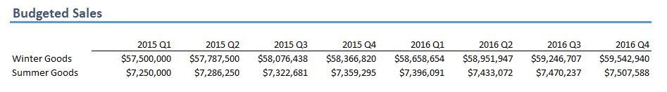
Mismatched Granularities
As a financial analyst, one problem I often have to solve is that of mismatched granularities. In our example, the actual sales data is shown to the category level, but let’s prepare a budget that is only on a seasonal level. To further this mismatch, we will prepare a quarterly budget, even through the sales data is daily.
Exhibit 11: Mismatched Granularities – Budget Table
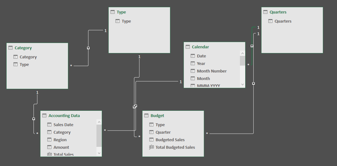
With Power Pivot for Excel, this inconsistency is easily solved. By creating two additional reference tables, or dimension tables in database nomenclature, we can now create the appropriate relationships to analyze our actual sales against the budgeted amounts.
Exhibit 12: Mismatched Granularities – Relationships
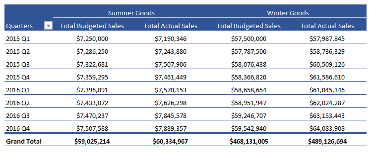
In Excel, the following PivotTable comes together quickly.
Exhibit 13: Mismatched Granularities – Budget vs. Actual Results
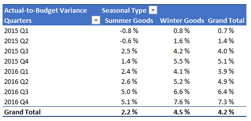
Further, we can define new measures that calculate the variance between actual sales and budgeted sales as below:
Actual-to-Budget Variance:=if(ISBLANK([Total Budgeted Sales]),BLANK(),[Total Sales]/[Total Budgeted Sales]-1)
Using this measure, we can show the variance on a PivotTable.
Exhibit 14: Mismatched Granularities – Variance Results